Envelope Deformation

Envelope Deformation

The code of Envelope Deformation uses the Bend Path code.

We first define four path parameters around the item bounding box: Top and Bottom, Left and Right. Each path represents a side of the deformation envelope and acts as a Bend Path effect.

Then the idea is to blend those four deformed paths is order to generate the final deformed path. To do this, we will use weighting: The closer a point is to a Bend Path, the more it will be affected by this Bend Path. So we had to find simple weight coefficients to use.

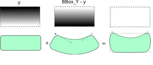
The first step is to blend the Top and the Bottom deformation. To do this, the rule is simple: the Top deformed path must be dominant for small y and the Bottom deformed path must be dominant for small (Bbox_y - y). We generate the blended path (named output-y) with the following formula:

(Bbox_y - y) * Deformation-Up + y * Deformation-Bottom

The following figure illustrates the process. It is important to notice that y + (Bbox_y - y) = constant. Indeed, we only have then to divide the result by Bbox_y to scale it to the original size.

Using the same model, the second step is to blend the Left and Right Deformations (we name it output-x).

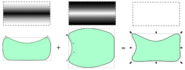
The final step uses the same method but is not as accurate as the previous operation. Indeed, in the end we will average two different results. Our first result is the calculation of output-1: The more a point is close to Top and Down, the less it will be affected by output-x. The following figure illustrates the process.

The weight coefficients used were y(Bbox_y - y) and (Bbox_y/4) - y(Bbox_y - y). We notice again that their sum is constant.

We then calculate output-2: The more a point is close to Left and Right, the less it will be affected by output-y. In the end, we do the mean between output-1 and output-2. Of course, from a mathematical point of view, the result is not perfect, but on a graphical one, we can consider that this is sufficient.